Distributed Hydrological Model Calibration #

The calibration of the Distributed rainfall runoff model follows the same steps of running the model with extra steps to define the calibration algorithm arguments

1- Catchment Object #

Import the Catchment object which is the main object in the distributed model, to read and check the input data, and when the model finish the simulation it stores the results and do the visualization

class Catchment:

    def __init__(self, name, StartDate, EndDate, fmt="%Y-%m-%d", SpatialResolution = 'Lumped',
                 TemporalResolution = "Daily"):
        """
        =============================================================================
            Catchment(name, StartDate, EndDate, fmt="%Y-%m-%d", SpatialResolution = 'Lumped',
                             TemporalResolution = "Daily")
        =============================================================================
        Parameters
        ----------
        name : [str]
            Name of the Catchment.
        StartDate : [str]
            starting date.
        EndDate : [str]
            end date.
        fmt : [str], optional
            format of the given date. The default is "%Y-%m-%d".
        SpatialResolution : TYPE, optional
            Lumped or 'Distributed' . The default is 'Lumped'.
        TemporalResolution : TYPE, optional
            "Hourly" or "Daily". The default is "Daily".
    """

- To instantiate the object you need to provide the name, statedate, enddate, and the SpatialResolution

from hapi.catchment import Catchment

start = "2009-01-01"
end = "2011-12-31"
name = "Coello"

Coello = Catchment(name, start, end, SpatialResolution = "Distributed")

Read Meteorological Inputs #

First define the directory where the data exist

Path = Comp + "/data/distributed/coello"
PrecPath = Path + "/prec"
Evap_Path = Path + "/evap"
TempPath = Path + "/temp"
FlowAccPath = Path + "/GIS/acc4000.tif"
FlowDPath = Path + "/GIS/fd4000.tif"
ParPathRun = Path + "/Parameter set-Avg/"

- Then use the each method in the object to read the coresponding data

Coello.read_rainfall(PrecPath)
Coello.read_temperature(TempPath)
Coello.read_et(Evap_Path)
Coello.read_flow_acc(FlowAccPath)
Coello.read_flow_dir(FlowDPath)

- To read the parameters you need to provide whether you need to consider the snow subroutine or not

Snow = 0
Coello.read_parameters(ParPathRun, Snow)

2- Lumped Model #

Get the Lumpde conceptual model you want to couple it with the distributed routing module which in our case HBV and define the initial condition, and catchment area.

from hapi.rrm.hbv_bergestrom92 import HBVBergestrom92 as HBV

CatchmentArea = 1530
InitialCond = [0,5,5,5,0]
Coello.read_lumped_model(HBV, CatchmentArea, InitialCond)

- If the Inpus are consistent in dimensions you will get a the following message

check_inputs

to check the performance of the model we need to read the gauge hydrographs

Coello.read_gauge_table("Hapi/Data/00inputs/Discharge/stations/gauges.csv", FlowAccPath)
GaugesPath = "Hapi/Data/00inputs/Discharge/stations/"
Coello.read_discharge_gauges(GaugesPath, column='id', fmt="%Y-%m-%d")

3-Run Object #

The Run object connects all the components of the simulation together, the Catchment object, the Lake object and the distributedrouting object
import the Run object and use the Catchment object as a parameter to the Run object, then call the RunHapi method to start the simulation

from hapi.run import Run
Run.RunHapi(Coello)

- the result of the simulation will be stored as attributes in the Catchment object as follow

"""
Outputs:
    1-statevariables: [numpy attribute]
        4D array (rows,cols,time,states) states are [sp,wc,sm,uz,lv]
    2-qlz: [numpy attribute]
        3D array of the lower zone discharge
    3-quz: [numpy attribute]
        3D array of the upper zone discharge
    4-qout: [numpy attribute]
        1D timeseries of discharge at the outlet of the catchment
        of unit m3/sec
    5-quz_routed: [numpy attribute]
        3D array of the upper zone discharge  accumulated and
        routed at each time step
    6-qlz_translated: [numpy attribute]
        3D array of the lower zone discharge translated at each time step
"""

4-Extract Hydrographs #

The final step is to extract the simulated Hydrograph from the cells at the location of the gauges to compare
The extract_discharge method extracts the hydrographs, however you have to provide in the gauge file the coordinates of the gauges with the same coordinate system of the FlowAcc raster

Coello.extract_discharge(factor=Coello.GaugesTable['area ratio'].tolist())

for i in range(len(Coello.GaugesTable)):
    gaugeid = Coello.GaugesTable.loc[i,'id']
    print("----------------------------------")
    print("Gauge - " +str(gaugeid))
    print("RMSE= " + str(round(Coello.Metrics.loc['RMSE',gaugeid],2)))
    print("NSE= " + str(round(Coello.Metrics.loc['NSE',gaugeid],2)))
    print("NSEhf= " + str(round(Coello.Metrics.loc['NSEhf',gaugeid],2)))
    print("KGE= " + str(round(Coello.Metrics.loc['KGE',gaugeid],2)))
    print("WB= " + str(round(Coello.Metrics.loc['WB',gaugeid],2)))
    print("Pearson CC= " + str(round(Coello.Metrics.loc['Pearson-CC',gaugeid],2)))
    print("R2 = " + str(round(Coello.Metrics.loc['R2',gaugeid],2)))

- The extract_discharge will print the performance metics

5-Visualization #

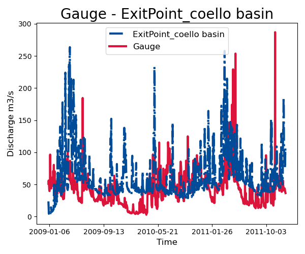
Firts type of visualization we can do with the results is to compare the gauge hydrograph with the simulatied hydrographs
Call the plot_hydrograph method and provide the period you want to visualize with the order of the gauge

gaugei = 5
plotstart = "2009-01-01"
plotend = "2011-12-31"

Coello.plot_hydrograph(plotstart, plotend, gaugei)

6-Animation #

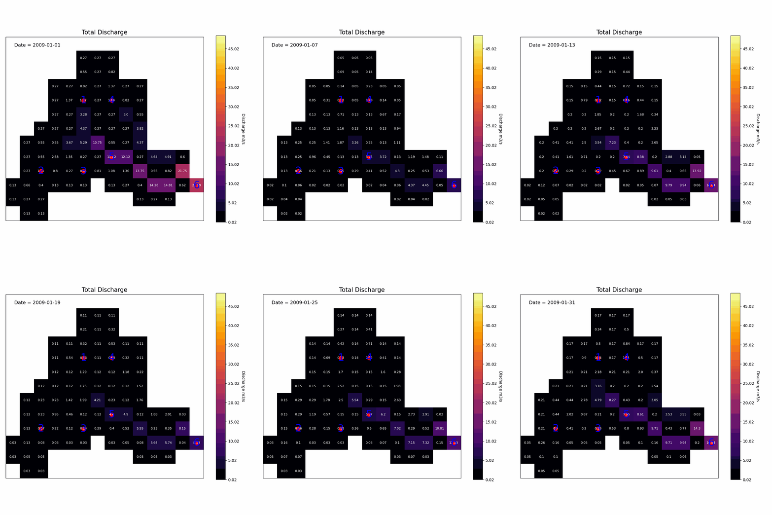
The best way to visualize a time series of distributed data is an animation. The Catchment object has a plot_distributed_results method which animates any of the model results.

The keyword arguments are forwarded to cleopatra.array_glyph.ArrayGlyph.animate; see its documentation for the full list. The commonly used ones are figsize, interval, cmap, ticks_spacing, color_scale ("linear", "power", "sym-lognorm", "boundary-norm", "midpoint"), display_cell_value, background_color_threshold, text_loc, point_color, pid_color and pid_size.

option selects the variable to animate:

option	variable	option	variable
1	Total discharge	7	Lower zone
2	Upper zone discharge	8	Water content
3	Ground water	9	Precipitation
4	Snow pack	10	Evapotranspiration
5	Soil moisture	11	Temperature
6	Upper zone

plotstart = "2009-01-01"
plotend = "2009-04-20"

anim = Coello.plot_distributed_results(
    plotstart,
    plotend,
    option=1,
    gauges=True,
    figsize=(9, 9),
    ticks_spacing=5,
    interval=200,
    cmap="inferno",
    color_scale="linear",
    display_cell_value=True,
    text_loc=[0.1, 0.2],
    point_color="red",
    pid_color="blue",
    pid_size=25,
)

To save the animation, the output format is taken from the file extension. GIF is written with Pillow; mov, avi and mp4 need FFmpeg installed and available on your system.

Coello.save_animation("results/anim.gif", fps=2)

7-Save the result into rasters #

To save the results as rasters provide the period and the path

start = "2009-01-01"
end = "2010-04-20"
prefix = "Qtot_"

Coello.save_results(
    FlowAccPath,
    result=1,
    start=start,
    end=end,
    path="results/",
    prefix=prefix,
)