Styles Module#
The styles module provides classes and functions for styling plots, including line styles, marker styles, scaling functions, and color normalization.
Styles Class#
cleopatra.styles.Styles
#
A class providing line and marker styles for matplotlib plots.
This class contains collections of predefined line styles and marker styles that can be used to customize matplotlib plots. It provides static methods to retrieve these styles by name or index.
Attributes:
| Name | Type | Description |
|---|---|---|
line_styles |
A dictionary of line style definitions, mapping style names to matplotlib line style tuples. Each tuple defines the line style pattern. |
|
marker_style_list |
A list of marker style strings that combine line styles with markers. |
Methods:
| Name | Description |
|---|---|
get_line_style |
Get a line style tuple by name or index. |
get_marker_style |
Get a marker style string by index. |
Notes
Line styles define the pattern of the line (solid, dashed, dotted, etc.), while marker styles define both the line pattern and the marker shape (circle, square, triangle, etc.) used at data points.
Examples:
>>> from cleopatra.styles import Styles
>>> # Get a line style by name
>>> solid_line = Styles.get_line_style("solid")
>>> # Get a line style by index
>>> dashed_line = Styles.get_line_style(5)  # "dashed"
>>> # Get a marker style
>>> marker_style = Styles.get_marker_style(0)  # "--o"
Source code in src/cleopatra/styles.py
129 130 131 132 133 134 135 136 137 138 139 140 141 142 143 144 145 146 147 148 149 150 151 152 153 154 155 156 157 158 159 160 161 162 163 164 165 166 167 168 169 170 171 172 173 174 175 176 177 178 179 180 181 182 183 184 185 186 187 188 189 190 191 192 193 194 195 196 197 198 199 200 201 202 203 204 205 206 207 208 209 210 211 212 213 214 215 216 217 218 219 220 221 222 223 224 225 226 227 228 229 230 231 232 233 234 235 236 237 238 239 240 241 242 243 244 245 246 247 248 249 250 251 252 253 254 255 256 257 258 259 260 261 262 263 264 265 266 267 268 269 270 271 272 273 274 275 276 277 278 279 280 281 282 283 284 285 286 287 288 289 290 291 292 293 294 295 296 297 298 299 300 301 302 303 304 305 306 307 308 309 310 311 312 313 314 315 316 317 318 319 320 321 322 323 324 325 326 327 328 329 330 331 332 333 334 335 | |
get_line_style(style='loosely dotted')
staticmethod
#
Get a matplotlib line style tuple by name or index.
This method retrieves a line style tuple that can be used with matplotlib plotting functions to customize the appearance of lines. The style can be specified either by name (string) or by index (integer).
Parameters:
| Name | Type | Description | Default |
|---|---|---|---|
style
|
str | int
|
The line style to retrieve, by default "loosely dotted".
If a string, it should be one of the keys in the |
'loosely dotted'
|
Returns:
| Type | Description |
|---|---|
tuple[int, tuple[int, ...]] | None
|
A matplotlib line style tuple that can be used with plot functions. |
tuple[int, tuple[int, ...]] | None
|
The tuple format is (offset, (on_off_seq)) where: |
tuple[int, tuple[int, ...]] | None
|
|
tuple[int, tuple[int, ...]] | None
|
|
Raises:
| Type | Description |
|---|---|
KeyError
|
If the style name provided does not exist in the |
Examples: Get a line style by name:
>>> from cleopatra.styles import Styles
>>> solid = Styles.get_line_style("solid")
>>> solid
(0, ())
>>> import matplotlib.pyplot as plt
>>> import numpy as np
>>> x = np.linspace(0, 10, 100)
>>> y = np.sin(x)
>>> plt.plot(x, y, linestyle=Styles.get_line_style("dashed"))  # doctest: +SKIP
Source code in src/cleopatra/styles.py
196 197 198 199 200 201 202 203 204 205 206 207 208 209 210 211 212 213 214 215 216 217 218 219 220 221 222 223 224 225 226 227 228 229 230 231 232 233 234 235 236 237 238 239 240 241 242 243 244 245 246 247 248 249 250 251 252 253 254 255 256 257 258 259 260 261 262 263 264 265 266 267 268 269 270 271 272 | |
get_marker_style(style)
staticmethod
#
Get a matplotlib marker style string by index.
This method retrieves a marker style string that can be used with matplotlib
plotting functions to customize the appearance of markers and lines. The style
is specified by an index into the marker_style_list.
Parameters:
| Name | Type | Description | Default |
|---|---|---|---|
style
|
int
|
The index of the marker style to retrieve from the |
required |
Returns:
| Name | Type | Description |
|---|---|---|
str
|
A matplotlib marker style string that combines line style and marker. |
|
Examples |
str
|
"--o" (dashed line with circle markers), ":D" (dotted line with |
str
|
diamond markers), etc. |
Notes
The marker style strings use matplotlib's shorthand notation: - Line styles: "-" (solid), "--" (dashed), "-." (dash-dot), ":" (dotted) - Markers: "o" (circle), "D" (diamond), "s" (square), "^" (triangle up), etc.
Examples: Get a marker style by index:
>>> from cleopatra.styles import Styles
>>> # Get the first marker style
>>> style0 = Styles.get_marker_style(0)
>>> style0
'--o'

>>> # Get another marker style
>>> style1 = Styles.get_marker_style(1)
>>> style1
':D'
>>> # If we have 11 styles and request index 15, we get style at index 15 % 11 = 4
>>> len(Styles.marker_style_list)
11
>>> style15 = Styles.get_marker_style(15)  # Same as style4
>>> style4 = Styles.get_marker_style(4)
>>> style15 == style4
True
>>> import matplotlib.pyplot as plt
>>> import numpy as np
>>> x = np.linspace(0, 10, 20)
>>> y = np.sin(x)
>>> plt.plot(x, y, Styles.get_marker_style(0))  # doctest: +SKIP
Source code in src/cleopatra/styles.py
Scale Class#
cleopatra.styles.Scale
#
A class providing various scaling functions for data visualization.
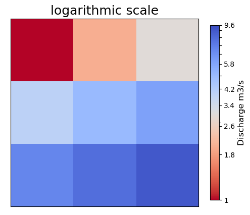
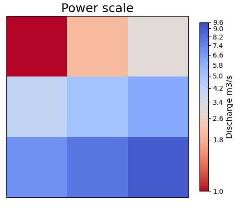
This class contains static methods for different types of scaling operations that can be used to transform data values for visualization purposes. These include logarithmic scaling, power scaling, identity scaling, and general value rescaling between different ranges.
Methods:
| Name | Description |
|---|---|
log_scale |
Apply logarithmic (base 10) scaling to a value. |
power_scale |
Create a power scaling function based on a minimum value. |
identity_scale |
Create an identity scaling function that always returns 2. |
rescale |
Rescale a value from one range to another. |
Notes
Scaling functions are useful for transforming data to improve visualization, especially when dealing with data that spans multiple orders of magnitude or needs to be normalized to a specific range.
Examples:
Apply logarithmic scaling:
>>> from cleopatra.styles import Scale
>>> Scale.log_scale(100)
np.float64(2.0)
>>> Scale.log_scale(1000)
np.float64(3.0)
>>> Scale.rescale(5, 0, 10, 0, 100)  # 5 is 50% of [0,10], so 50% of [0,100] is 50
50.0
>>> Scale.rescale(75, 0, 100, -1, 1)  # 75 is 75% of [0,100], so 75% of [-1,1] is 0.5
0.5
Source code in src/cleopatra/styles.py
338 339 340 341 342 343 344 345 346 347 348 349 350 351 352 353 354 355 356 357 358 359 360 361 362 363 364 365 366 367 368 369 370 371 372 373 374 375 376 377 378 379 380 381 382 383 384 385 386 387 388 389 390 391 392 393 394 395 396 397 398 399 400 401 402 403 404 405 406 407 408 409 410 411 412 413 414 415 416 417 418 419 420 421 422 423 424 425 426 427 428 429 430 431 432 433 434 435 436 437 438 439 440 441 442 443 444 445 446 447 448 449 450 451 452 453 454 455 456 457 458 459 460 461 462 463 464 465 466 467 468 469 470 471 472 473 474 475 476 477 478 479 480 481 482 483 484 485 486 487 488 489 490 491 492 493 494 495 496 497 498 499 500 501 502 503 504 505 506 507 508 509 510 511 512 513 514 515 516 517 518 519 520 521 522 523 524 525 526 527 528 529 530 531 532 533 534 535 536 537 538 539 540 541 542 543 544 545 546 547 548 549 550 551 552 553 554 555 556 557 558 559 560 561 562 563 564 565 566 567 568 569 570 571 572 573 574 575 576 577 578 579 580 581 582 583 584 585 586 587 588 589 590 591 592 593 594 595 596 | |
__init__()
#
Initialize a Scale object.
Note that this class is primarily intended to be used via its static methods, so initialization is not typically necessary.
identity_scale(min_val, max_val)
staticmethod
#
Create a constant scaling function that always returns 2.
This method returns a function that ignores its input and always returns the constant value 2. Despite its name, this is not a true identity function (which would return the input unchanged), but rather a constant function.
Parameters:
| Name | Type | Description | Default |
|---|---|---|---|
min_val
|
float
|
The minimum value in the data range. This parameter is not used in the implementation but is included for API consistency with other scaling methods. |
required |
max_val
|
float
|
The maximum value in the data range. This parameter is not used in the implementation but is included for API consistency with other scaling methods. |
required |
Returns:
| Type | Description |
|---|---|
Callable
|
A function that takes any input and always returns 2. |
Callable
|
The returned function has the signature: f(val) -> int |
Notes
This function can be useful in situations where: - A constant size or value is needed regardless of the input data - A placeholder scaling function is required - Testing or debugging code that expects a scaling function
Examples: Create and use the constant scaling function:
>>> from cleopatra.styles import Scale
>>> scale_func = Scale.identity_scale(0, 100)  # min_val and max_val are ignored
>>> scale_func(5)  # Returns 2 regardless of input
2
>>> scale_func(100)  # Still returns 2
2
>>> scale_func(-10)  # Still returns 2
2
>>> import numpy as np
>>> values = np.array([1, 2, 3, 4, 5])
>>> scale_func(values)  # Returns scalar 2, not an array of 2s
2
Source code in src/cleopatra/styles.py
log_scale(val)
staticmethod
#
Apply logarithmic (base 10) scaling to a value or array.
This method computes the base-10 logarithm of the input value(s), which is useful for visualizing data that spans multiple orders of magnitude.
Parameters:
| Name | Type | Description | Default |
|---|---|---|---|
val
|
float | ndarray
|
The value or array of values to be logarithmically scaled. Must be positive (greater than 0) to avoid math domain errors. |
required |
Returns:
| Type | Description |
|---|---|
floating | ndarray
|
The base-10 logarithm of the input value(s). |
floating | ndarray
|
If the input is an array, the output will be an array of the same shape. |
Notes
Logarithmic scaling is particularly useful for: - Data that spans multiple orders of magnitude - Compressing wide ranges of values into a more manageable range - Visualizing exponential growth or decay
Examples: Scale a single value:
>>> from cleopatra.styles import Scale
>>> Scale.log_scale(100)
np.float64(2.0)
>>> Scale.log_scale(1000)
np.float64(3.0)
>>> import numpy as np
>>> values = np.array([1, 10, 100, 1000])
>>> Scale.log_scale(values)
array([0., 1., 2., 3.])
Source code in src/cleopatra/styles.py
power_scale(min_val)
staticmethod
#
Create a power scaling function based on a minimum value.
This method returns a function that applies power scaling to its input. The scaling function first shifts the input value by adding the absolute value of the minimum value plus 1 (to ensure positive values), then divides by 1000 and squares the result.
Parameters:
| Name | Type | Description | Default |
|---|---|---|---|
min_val
|
float
|
The minimum value in the data range. Used to shift the data to ensure all values are positive before applying the power transformation. |
required |
Returns:
| Type | Description |
|---|---|
Callable
|
A function that takes a value or array and returns the power-scaled result. |
Callable
|
The returned function has the signature: f(val) -> float or numpy.ndarray |
Notes
Power scaling is useful for: - Emphasizing differences in smaller values - Compressing the range of larger values - Creating non-linear visualizations where small changes in small values are more important than small changes in large values
Examples: Create a power scaling function and apply it to values:
>>> from cleopatra.styles import Scale
>>> # Create a scaling function with minimum value -10
>>> scale_func = Scale.power_scale(-10)
>>> # Apply to a single value
>>> scale_func(5)  # (5 + |-10| + 1) / 1000)^2 = (5 + 10 + 1)^2 / 1000000 = 16^2 / 1000000 = 256 / 1000000 = 0.000256
0.000256
>>> # Apply to another value
>>> scale_func(100)  # (100 + |-10| + 1) / 1000)^2 = (100 + 10 + 1)^2 / 1000000 = 111^2 / 1000000 = 12321 / 1000000 ≈ 0.012321
0.012321
>>> import numpy as np
>>> values = np.array([0, 10, 100])
>>> scale_func = Scale.power_scale(-5)
>>> scale_func(values)  # doctest: +ELLIPSIS
array([3.6000e-05, 2.5600e-04, 1.1236e-02])

>>> # [(0+5+1)/1000]^2, [(10+5+1)/1000]^2, [(100+5+1)/1000]^2]
Source code in src/cleopatra/styles.py
rescale(old_value, old_min, old_max, new_min, new_max)
staticmethod
#
Rescale a value from one range to another.
This method performs linear rescaling of a value from an original range [old_min, old_max] to a new range [new_min, new_max]. The transformation preserves the relative position of the value within its range.
Parameters:
| Name | Type | Description | Default |
|---|---|---|---|
old_value
|
float | ndarray
|
The value(s) to be rescaled. Can be a single value or an array. |
required |
old_min
|
float
|
The minimum value of the original range. |
required |
old_max
|
float
|
The maximum value of the original range. |
required |
new_min
|
float
|
The minimum value of the target range. |
required |
new_max
|
float
|
The maximum value of the target range. |
required |
Returns:
| Type | Description |
|---|---|
float | ndarray
|
The rescaled value(s) in the new range. If the input is an array, |
float | ndarray
|
the output will be an array of the same shape. |
Notes
The rescaling formula is: new_value = (((old_value - old_min) * (new_max - new_min)) / (old_max - old_min)) + new_min
This function is useful for: - Normalizing data to a specific range (e.g., [0, 1]) - Converting between different units or scales - Preparing data for visualization with specific bounds
Examples: Rescale a value from [0, 10] to [0, 100]:
>>> from cleopatra.styles import Scale
>>> Scale.rescale(5, 0, 10, 0, 100)  # 5 is 50% of [0,10], so 50% of [0,100] is 50
50.0
>>> import numpy as np
>>> values = np.array([0, 5, 10])
>>> Scale.rescale(values, 0, 10, 0, 1)  # Normalize to [0,1]
array([0. , 0.5, 1. ])
Source code in src/cleopatra/styles.py
ColorScale Enum#
ColorScale is the StrEnum of accepted color_scale values — linear / power /
sym-lognorm / boundary-norm / midpoint. Members are real strings (so
ColorScale.LINEAR == "linear") and lookup is case-insensitive. ArrayGlyph /
MeshGlyph coerce color_scale through it, so an unrecognised value (or a non-string
such as an int) raises a clear ValueError instead of an obscure AttributeError. It is
also re-exported from cleopatra.array_glyph.
cleopatra.styles.ColorScale
#
Bases: StrEnum
Accepted values for the color_scale option of cleopatra glyphs.
Members are plain strings (StrEnum), so ColorScale.LINEAR == "linear"
holds and any code that treats the value as a string keeps working
whether the caller passes the enum member or the bare string. Lookup is
case-insensitive: ColorScale("Linear") is ColorScale.LINEAR.
Examples:
- The members behave like their string values:
- Construction is case-insensitive; bad values raise
ValueError:
Source code in src/cleopatra/styles.py
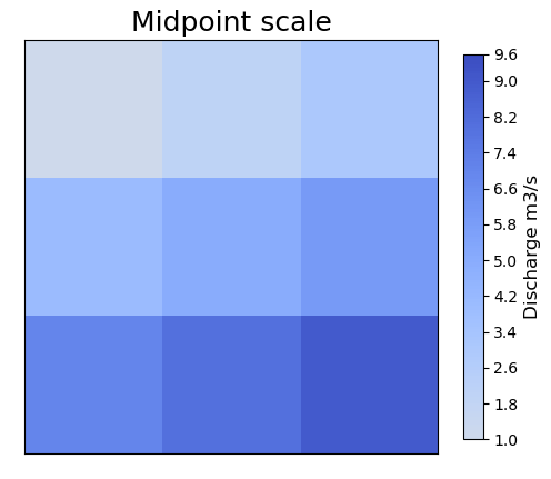
MidpointNormalize Class#
cleopatra.styles.MidpointNormalize
#
Bases: Normalize
A normalization class that scales data with a midpoint.
This class extends matplotlib's Normalize class to create a colormap normalization that has a fixed midpoint. This is useful for data that has a natural midpoint (like zero) where the colormap should be centered, regardless of the actual data range.
The normalization maps values to the range [0, 1] with the midpoint mapped to 0.5, which allows for symmetric colormaps to be properly centered.
Parameters:
| Name | Type | Description | Default |
|---|---|---|---|
vmin
|
float | None
|
The minimum data value that corresponds to 0 in the normalized data. If None, it is automatically calculated from the data. |
None
|
vmax
|
float | None
|
The maximum data value that corresponds to 1 in the normalized data. If None, it is automatically calculated from the data. |
None
|
midpoint
|
float | None
|
The data value that corresponds to 0.5 in the normalized data. If None, it defaults to the midpoint between vmin and vmax. |
None
|
clip
|
bool
|
If True, values outside the [vmin, vmax] range are clipped to be within that range, by default False. |
False
|
Attributes:
| Name | Type | Description |
|---|---|---|
midpoint |
The data value that will be mapped to 0.5 in the normalized data. |
Notes
This normalization is particularly useful for: - Diverging colormaps where a specific value should be at the center - Data with positive and negative values where zero should be the midpoint - Highlighting deviations from a reference value
Examples: Create a plot with a midpoint normalization:
>>> import numpy as np
>>> import matplotlib.pyplot as plt
>>> from cleopatra.styles import MidpointNormalize
>>> # Create some data with positive and negative values
>>> data = np.linspace(-10, 10, 100)
>>> # Create a normalization with midpoint at 0
>>> norm = MidpointNormalize(vmin=-10, vmax=10, midpoint=0)
>>> # Use in a plot
>>> plt.figure(figsize=(8, 1)) # doctest: +SKIP
>>> plt.imshow([data], cmap='coolwarm', norm=norm, aspect='auto')  # doctest: +SKIP
>>> plt.colorbar()  # doctest: +SKIP
>>> plt.title('Midpoint Normalization with midpoint=0')  # doctest: +SKIP
>>> plt.tight_layout()  # doctest: +SKIP
>>> norm(0)
masked_array(data=0.,
             mask=False,
       fill_value=1e+20)
>>> norm(2.5)
masked_array(data=0.25,
             mask=False,
       fill_value=1e+20)
>>> norm(7.5)
masked_array(data=0.75,
             mask=False,
       fill_value=1e+20)
>>> norm(10)
masked_array(data=1.,
             mask=False,
       fill_value=1e+20)
Source code in src/cleopatra/styles.py
715 716 717 718 719 720 721 722 723 724 725 726 727 728 729 730 731 732 733 734 735 736 737 738 739 740 741 742 743 744 745 746 747 748 749 750 751 752 753 754 755 756 757 758 759 760 761 762 763 764 765 766 767 768 769 770 771 772 773 774 775 776 777 778 779 780 781 782 783 784 785 786 787 788 789 790 791 792 793 794 795 796 797 798 799 800 801 802 803 804 805 806 807 808 809 810 811 812 813 814 815 816 817 818 819 820 821 822 823 824 825 826 827 828 829 830 831 832 833 834 835 836 837 838 839 840 841 842 843 844 845 846 847 848 849 850 851 852 853 854 855 856 857 858 859 860 861 862 863 864 865 866 867 868 869 870 871 872 873 874 875 876 877 878 879 880 881 882 883 884 885 886 887 888 889 890 891 892 893 894 895 896 897 898 899 900 901 902 903 904 905 906 907 908 909 910 911 912 913 914 915 916 917 918 919 | |
__call__(value, clip=None)
#
Normalize data values to the [0, 1] range with a fixed midpoint.
This method implements the normalization logic, mapping input values to the range [0, 1] with the midpoint mapped to 0.5. It uses linear interpolation to create two separate linear mappings: one for values below the midpoint and another for values above the midpoint.
Parameters:
| Name | Type | Description | Default |
|---|---|---|---|
value
|
float | ndarray
|
The data value(s) to normalize. Can be a single value or an array. |
required |
clip
|
bool | None
|
Whether to clip the input values to the [vmin, vmax] range. If None, the clip attribute of the instance is used. |
None
|
Returns:
| Type | Description |
|---|---|
MaskedArray
|
The normalized value(s) in the range [0, 1], with the midpoint mapped to 0.5. |
MaskedArray
|
If the input is an array, the output will be an array of the same shape. |
MaskedArray
|
Masked values in the input remain masked in the output. |
Notes
The normalization is performed using numpy's interp function, which does linear interpolation between the points: - (vmin, 0): minimum value maps to 0 - (midpoint, 0.5): midpoint value maps to 0.5 - (vmax, 1): maximum value maps to 1
This creates a piecewise linear mapping that ensures the midpoint is always at 0.5 in the normalized range.
Examples: - Normalize values with a zero midpoint:
>>> from cleopatra.styles import MidpointNormalize
>>> norm = MidpointNormalize(vmin=-10, vmax=10, midpoint=0)
>>> # Values below midpoint are mapped to [0, 0.5]
>>> norm(-10)  # vmin maps to 0
masked_array(data=0.,
             mask=False,
       fill_value=1e+20)
>>> norm(-5)   # halfway between vmin and midpoint maps to 0.25
masked_array(data=0.25,
             mask=False,
       fill_value=1e+20)
>>> norm(5)    # halfway between midpoint and vmax maps to 0.75
masked_array(data=0.75,
             mask=False,
       fill_value=1e+20)
>>> norm(10)   # vmax maps to 1
masked_array(data=1.,
             mask=False,
       fill_value=1e+20)
>>> import numpy as np
>>> values = np.array([-10, -5, 0, 5, 10])
>>> norm(values)
masked_array(data=[0.  , 0.25, 0.5 , 0.75, 1.  ],
             mask=False,
       fill_value=1e+20)
Source code in src/cleopatra/styles.py
840 841 842 843 844 845 846 847 848 849 850 851 852 853 854 855 856 857 858 859 860 861 862 863 864 865 866 867 868 869 870 871 872 873 874 875 876 877 878 879 880 881 882 883 884 885 886 887 888 889 890 891 892 893 894 895 896 897 898 899 900 901 902 903 904 905 906 907 908 909 910 911 912 913 914 915 916 917 918 919 | |
__init__(vmin=None, vmax=None, midpoint=None, clip=False)
#
Initialize a MidpointNormalize instance.
Parameters:
| Name | Type | Description | Default |
|---|---|---|---|
vmin
|
float | None
|
The minimum data value that corresponds to 0 in the normalized data. If None, it is automatically calculated from the data when the normalization is applied. |
None
|
vmax
|
float | None
|
The maximum data value that corresponds to 1 in the normalized data. If None, it is automatically calculated from the data when the normalization is applied. |
None
|
midpoint
|
float | None
|
The data value that corresponds to 0.5 in the normalized data. If None, it defaults to the midpoint between vmin and vmax. |
None
|
clip
|
bool
|
If True, values outside the [vmin, vmax] range are clipped to be within that range, by default False. |
False
|
Notes
This initialization sets up the midpoint attribute and calls the parent class (matplotlib.colors.Normalize) constructor with the vmin, vmax, and clip parameters.
Examples: Create a normalization with default parameters:
>>> from cleopatra.styles import MidpointNormalize
>>> norm = MidpointNormalize()  # vmin, vmax, midpoint will be determined from data
Source code in src/cleopatra/styles.py
Classification — classify#
classify bins a continuous array into discrete colour classes, returning the
bin edges and a matplotlib BoundaryNorm. It is the shared building block behind
classified (categorical) colouring. All schemes are NumPy-native (no extra
dependency): "quantiles", "equal_interval", "percentiles", "std_mean",
and the Jenks-family "fisher_jenks" / "natural_breaks". A non-string scheme
is treated as explicit, already-chosen bin edges.
cleopatra.styles.classify(values, scheme, k=5)
#
Bin a continuous array into discrete colour classes.
The shared building block behind categorical (classified) colouring:
it turns a continuous data column into an array of bin edges plus a
matching matplotlib.colors.BoundaryNorm, so any colour-by-value glyph
can render a stepped colorbar / class legend instead of a continuous
ramp. It is the classification counterpart to Scale and
MidpointNormalize.
The numpy-only schemes (no dependency beyond numpy) are:
"quantiles"—kequal-count classes vianp.quantile(values, np.linspace(0, 1, k + 1))."equal_interval"—kequal-width classes spanning the data range."percentiles"—kequal-count classes vianp.percentileon the same evenly-spaced probabilities; numerically equivalent to"quantiles"(it differs only in the[0, 100]vs[0, 1]convention) and is kept as a familiar alias."std_mean"— fixed breaks atmean + nσfornin(-2, -1, 0, 1, 2), clipped to the data range.kis ignored for this scheme (the number of classes follows from the multiples).
The Jenks-family schemes "fisher_jenks" and "natural_breaks" are
computed by the native Fisher-Jenks optimisation — the exact dynamic
program that minimises the within-class sum of squared deviations. Both
names are aliases for the same algorithm. No dependency beyond numpy.
A non-string scheme is treated as an explicit, already-chosen
sequence of bin edges (sorted ascending); k is ignored.
Parameters:
| Name | Type | Description | Default |
|---|---|---|---|
values
|
ndarray | Sequence[float]
|
The data to classify. Non-finite entries ( |
required |
scheme
|
str | Sequence[float]
|
A scheme name (see above, case-insensitive) or an explicit sequence of bin edges to use verbatim. |
required |
k
|
int
|
The number of classes for the count/width schemes. Must be
|
5
|
Returns:
| Type | Description |
|---|---|
tuple[ndarray, BoundaryNorm]
|
tuple[np.ndarray, matplotlib.colors.BoundaryNorm]: The sorted,
de-duplicated bin edges (length = classes + 1) and a
|
Raises:
| Type | Description |
|---|---|
ValueError
|
If |
Examples:
- Equal-interval edges on a 0–10 ramp:
- Quantile edges put equal counts in each class:
- An explicit edge sequence is used verbatim (sorted):
- An unknown scheme name is rejected:
Source code in src/cleopatra/styles.py
1350 1351 1352 1353 1354 1355 1356 1357 1358 1359 1360 1361 1362 1363 1364 1365 1366 1367 1368 1369 1370 1371 1372 1373 1374 1375 1376 1377 1378 1379 1380 1381 1382 1383 1384 1385 1386 1387 1388 1389 1390 1391 1392 1393 1394 1395 1396 1397 1398 1399 1400 1401 1402 1403 1404 1405 1406 1407 1408 1409 1410 1411 1412 1413 1414 1415 1416 1417 1418 1419 1420 1421 1422 1423 1424 1425 1426 1427 1428 1429 1430 1431 1432 1433 1434 1435 1436 1437 1438 1439 1440 1441 1442 1443 1444 1445 1446 1447 1448 1449 1450 1451 1452 1453 1454 1455 1456 1457 1458 1459 1460 1461 1462 1463 1464 1465 1466 1467 1468 1469 1470 | |
Value → size — resolve_sizes#
resolve_sizes maps per-item magnitudes to a visual size range — the reusable
value→size primitive shared by the size-encoding glyphs (ScatterGlyph marker
areas, FlowGlyph line widths).
cleopatra.styles.resolve_sizes(values, out_min, out_max, scale='linear')
#
Map per-item magnitudes to a visual size range.
The reusable value→size primitive shared by size-encoding glyphs: it
turns a per-item magnitude array into an array of visual sizes spanning
[out_min, out_max], optionally pre-transforming the magnitudes
("log" / "sqrt") before the linear rescale. ScatterGlyph uses it
for marker area (s); a future FlowGlyph can reuse it for line width.
The linear rescale itself is delegated to Scale.rescale, so this never
re-implements the range mapping.
The mapping is monotonic in the input, so larger magnitudes always map to larger sizes. When every (finite) magnitude is equal, there is no spread to encode and the midpoint of the output range is returned for each item.
Parameters:
| Name | Type | Description | Default |
|---|---|---|---|
values
|
ndarray | Sequence[float]
|
The per-item magnitudes to map. Must be finite — a
non-finite entry ( |
required |
out_min
|
float
|
The smallest output size (maps to the minimum magnitude). |
required |
out_max
|
float
|
The largest output size (maps to the maximum magnitude). |
required |
scale
|
str
|
The pre-transform: |
'linear'
|
Returns:
| Type | Description |
|---|---|
ndarray
|
np.ndarray: The mapped sizes, the same shape as |
Raises:
| Type | Description |
|---|---|
ValueError
|
If |
Examples:
- Linear mapping spans the output range, smallest→
out_min: - The mapping is monotonic, so ranking is preserved:
- All-equal magnitudes map to the output midpoint:
Source code in src/cleopatra/styles.py
606 607 608 609 610 611 612 613 614 615 616 617 618 619 620 621 622 623 624 625 626 627 628 629 630 631 632 633 634 635 636 637 638 639 640 641 642 643 644 645 646 647 648 649 650 651 652 653 654 655 656 657 658 659 660 661 662 663 664 665 666 667 668 669 670 671 672 673 674 675 676 677 678 679 680 681 682 683 684 685 686 687 688 689 690 691 692 693 694 695 696 697 698 699 700 701 702 703 704 705 706 707 708 709 710 711 712 | |
Legend builders#
Reusable, glyph-independent legend helpers that attach a legend to any Axes:
disjoint_legend— a categorical (disjoint) swatch legend.size_legend— a legend whose marker sizes encode magnitude.width_legend— a legend whose line widths encode magnitude.colorbar_legend— attach a colorbar for aScalarMappable.histogram_legend— a colour-mapped histogram drawn as a compact legend.
cleopatra.styles.disjoint_legend(ax, colors, labels, *, edgecolor='none', **kwargs)
#
Attach a categorical (disjoint) swatch legend to an axes.
Builds one filled rectangle (matplotlib.patches.Patch) per
category and registers them as a legend on ax. This is the
discrete counterpart to a colorbar: use it when categories are
nominal/disjoint (land-cover classes, region names, ...) rather
than samples of a continuous scale, where a colorbar would imply a
false ordering.
Parameters:
| Name | Type | Description | Default |
|---|---|---|---|
ax
|
Axes
|
The axes the legend is attached to. |
required |
colors
|
Sequence
|
One color per category, in any matplotlib color form
(name, hex, or RGB(A) tuple). Must be the same length as
|
required |
labels
|
Sequence[str]
|
The category label drawn next to each swatch. Must be
the same length as |
required |
edgecolor
|
str
|
Outline color for every swatch. Defaults to
|
'none'
|
**kwargs
|
Forwarded verbatim to |
{}
|
Returns:
| Name | Type | Description |
|---|---|---|
Legend |
Legend
|
The created legend artist, already added to |
Raises:
| Type | Description |
|---|---|
ValueError
|
If |
Examples:
- Build a three-class legend and read back its labels:
>>> import matplotlib.pyplot as plt >>> from cleopatra.styles import disjoint_legend >>> fig, ax = plt.subplots() >>> legend = disjoint_legend( ... ax, ... ["#1b9e77", "#d95f02", "#7570b3"], ... ["water", "urban", "forest"], ... ) >>> [t.get_text() for t in legend.get_texts()] ['water', 'urban', 'forest'] - Forward
Axes.legendkwargs such as a title and column count: - Mismatched lengths raise
ValueError:
Source code in src/cleopatra/styles.py
922 923 924 925 926 927 928 929 930 931 932 933 934 935 936 937 938 939 940 941 942 943 944 945 946 947 948 949 950 951 952 953 954 955 956 957 958 959 960 961 962 963 964 965 966 967 968 969 970 971 972 973 974 975 976 977 978 979 980 981 982 983 984 985 986 987 988 989 990 991 992 993 994 995 996 997 998 999 1000 1001 1002 1003 1004 1005 1006 1007 | |
cleopatra.styles.size_legend(ax, marker_sizes, labels, *, color='0.4', marker='o', **kwargs)
#
Attach a legend whose marker sizes encode magnitude.
The size counterpart to disjoint_legend: where that varies the swatch
colour, this varies the marker size, so it is the right legend for a
bubble / size-scaled scatter (e.g. ScatterGlyph(..., sizes=...)). One
proxy marker is drawn per entry, sized to match the points it
represents.
marker_sizes are scatter-style areas (points², the same unit as a
glyph's resolved s); each is converted to the matplotlib Line2D
markersize (a diameter in points) via sqrt, so the swatches match
the plotted points visually.
Parameters:
| Name | Type | Description | Default |
|---|---|---|---|
ax
|
Axes
|
The axes the legend is attached to. |
required |
marker_sizes
|
Sequence[float]
|
The representative marker areas (points²), one per
legend entry. Must be the same length as |
required |
labels
|
Sequence[str]
|
The text drawn next to each marker. Must be the same length
as |
required |
color
|
str
|
Fill colour for every proxy marker. Defaults to a neutral
grey ( |
'0.4'
|
marker
|
str
|
The marker style for the proxies. Defaults to |
'o'
|
**kwargs
|
Forwarded verbatim to |
{}
|
Returns:
| Name | Type | Description |
|---|---|---|
Legend |
Legend
|
The created legend artist, already added to |
Raises:
| Type | Description |
|---|---|
ValueError
|
If |
Examples:
- Build a three-entry size legend and read back its labels:
- Larger areas produce larger proxy markers (diameters in points):
Source code in src/cleopatra/styles.py
1010 1011 1012 1013 1014 1015 1016 1017 1018 1019 1020 1021 1022 1023 1024 1025 1026 1027 1028 1029 1030 1031 1032 1033 1034 1035 1036 1037 1038 1039 1040 1041 1042 1043 1044 1045 1046 1047 1048 1049 1050 1051 1052 1053 1054 1055 1056 1057 1058 1059 1060 1061 1062 1063 1064 1065 1066 1067 1068 1069 1070 1071 1072 1073 1074 1075 1076 1077 1078 1079 1080 1081 1082 1083 1084 1085 1086 1087 1088 1089 1090 1091 1092 1093 | |
cleopatra.styles.width_legend(ax, linewidths, labels, *, color='0.4', **kwargs)
#
Attach a legend whose line widths encode magnitude.
The line-width counterpart to size_legend (which varies marker size):
each entry is a short line drawn at the given linewidth, so it is the
right legend for a width-scaled flow / Sankey map
(e.g. FlowGlyph(..., widths=...)).
Parameters:
| Name | Type | Description | Default |
|---|---|---|---|
ax
|
Axes
|
The axes the legend is attached to. |
required |
linewidths
|
Sequence[float]
|
The representative line widths (points), one per legend
entry. Must be the same length as |
required |
labels
|
Sequence[str]
|
The text drawn next to each line. Must be the same length as
|
required |
color
|
str
|
Colour for every proxy line. Defaults to a neutral grey
( |
'0.4'
|
**kwargs
|
Forwarded verbatim to |
{}
|
Returns:
| Name | Type | Description |
|---|---|---|
Legend |
Legend
|
The created legend artist, already added to |
Raises:
| Type | Description |
|---|---|
ValueError
|
If |
Examples:
- Build a width legend and read back its labels:
- Larger magnitudes give thicker proxy lines:
Source code in src/cleopatra/styles.py
1096 1097 1098 1099 1100 1101 1102 1103 1104 1105 1106 1107 1108 1109 1110 1111 1112 1113 1114 1115 1116 1117 1118 1119 1120 1121 1122 1123 1124 1125 1126 1127 1128 1129 1130 1131 1132 1133 1134 1135 1136 1137 1138 1139 1140 1141 1142 1143 1144 1145 1146 1147 1148 1149 1150 1151 1152 1153 1154 1155 1156 1157 1158 1159 1160 1161 1162 | |
cleopatra.styles.colorbar_legend(mappable, ax=None, **kwargs)
#
Attach a continuous colorbar legend for a mappable.
A thin, glyph-agnostic wrapper over Figure.colorbar for callers
that already hold a mappable (the artist returned by
scatter / imshow / quiver / a glyph's plot) and just want a
matching colorbar. For full cleopatra colorbar styling (label size,
location, shrink) use Glyph.create_color_bar instead; this helper
is the minimal counterpart that sits alongside disjoint_legend
and histogram_legend.
Parameters:
| Name | Type | Description | Default |
|---|---|---|---|
mappable
|
ScalarMappable
|
A |
required |
ax
|
Axes
|
Axes to steal space from for the colorbar. Defaults to the mappable's own axes. The parent figure is inferred from whichever axes is used. |
None
|
**kwargs
|
Forwarded to |
{}
|
Returns:
| Name | Type | Description |
|---|---|---|
Colorbar |
Colorbar
|
The created colorbar. |
Raises:
| Type | Description |
|---|---|
ValueError
|
If no axes can be determined (the mappable is not
attached to an axes and |
Examples:
- Build a colorbar for a coloured scatter and read its label:
Source code in src/cleopatra/styles.py
cleopatra.styles.histogram_legend(ax, values=None, *, mappable=None, cmap=None, norm=None, bins=20, orientation='vertical', **bar_kwargs)
#
Draw a colour-mapped histogram as a distribution legend.
Renders a histogram of values whose bars are coloured by the same
colormap/norm used for the data, so the legend doubles as a
distribution plot — the third legend style alongside the continuous
colorbar and the categorical disjoint_legend. The colour mapping
can be taken straight from a mappable (so it matches a glyph's
plot exactly) or supplied explicitly via cmap / norm.
Parameters:
| Name | Type | Description | Default |
|---|---|---|---|
ax
|
Axes
|
Axes to draw the histogram on (typically a small companion axes beside the main plot). |
required |
values
|
ndarray | None
|
1D data to histogram. Non-finite entries are dropped.
Defaults to the mappable's array when |
None
|
mappable
|
ScalarMappable | None
|
Optional |
None
|
cmap
|
Colormap name or object. Falls back to the mappable's
cmap, then to matplotlib's default. Ignored when a
|
None
|
|
norm
|
Normalize | None
|
Normalization for mapping bin centres to colours. Falls back to the mappable's norm, then to a linear norm spanning the data. |
None
|
bins
|
int
|
Number of histogram bins. Default is 20. |
20
|
orientation
|
str
|
|
'vertical'
|
**bar_kwargs
|
Forwarded to |
{}
|
Returns:
| Name | Type | Description |
|---|---|---|
BarContainer |
BarContainer
|
The bars drawn, one per bin. |
Raises:
| Type | Description |
|---|---|
ValueError
|
If neither |
Examples:
- Histogram legend from explicit values and a colormap:
- Inherit cmap/norm/data straight from a mappable:
Source code in src/cleopatra/styles.py
1215 1216 1217 1218 1219 1220 1221 1222 1223 1224 1225 1226 1227 1228 1229 1230 1231 1232 1233 1234 1235 1236 1237 1238 1239 1240 1241 1242 1243 1244 1245 1246 1247 1248 1249 1250 1251 1252 1253 1254 1255 1256 1257 1258 1259 1260 1261 1262 1263 1264 1265 1266 1267 1268 1269 1270 1271 1272 1273 1274 1275 1276 1277 1278 1279 1280 1281 1282 1283 1284 1285 1286 1287 1288 1289 1290 1291 1292 1293 1294 1295 1296 1297 1298 1299 1300 1301 1302 1303 1304 1305 1306 1307 1308 1309 1310 1311 1312 1313 1314 1315 1316 1317 1318 1319 1320 1321 1322 1323 1324 1325 1326 | |
Examples#
Log Scale#
import numpy as np
import matplotlib.pyplot as plt
from cleopatra.styles import Scale

# Create some data with a wide range of values
data = np.array([0.1, 1, 10, 100, 1000])

# Apply log scale
scale = Scale()
log_data = scale.log_scale(data)

# Plot the original and log-scaled data
fig, (ax1, ax2) = plt.subplots(1, 2, figsize=(10, 4))
ax1.plot(data)
ax1.set_title('Original Data')
ax2.plot(log_data)
ax2.set_title('Log-Scaled Data')
plt.tight_layout()
Power Scale#
# Apply power scale with gamma=0.5 (square root)
power_data = scale.power_scale(data)(0.5)

# Plot the original and power-scaled data
fig, (ax1, ax2) = plt.subplots(1, 2, figsize=(10, 4))
ax1.plot(data)
ax1.set_title('Original Data')
ax2.plot(power_data)
ax2.set_title('Power-Scaled Data (gamma=0.5)')
plt.tight_layout()
Midpoint Normalize#
import numpy as np
import matplotlib.pyplot as plt
from cleopatra.styles import MidpointNormalize
import matplotlib.colors as colors

# Create some data with positive and negative values
data = np.random.uniform(-10, 10, (10, 10))

# Create a figure with two subplots
fig, (ax1, ax2) = plt.subplots(1, 2, figsize=(10, 4))

# Plot with standard normalization
im1 = ax1.imshow(data, cmap='RdBu_r', norm=colors.Normalize(vmin=-10, vmax=10))
ax1.set_title('Standard Normalization')
plt.colorbar(im1, ax=ax1)

# Plot with midpoint normalization (midpoint at 0)
im2 = ax2.imshow(data, cmap='RdBu_r', norm=MidpointNormalize(vmin=-10, vmax=10, midpoint=0))
ax2.set_title('Midpoint Normalization')
plt.colorbar(im2, ax=ax2)

plt.tight_layout()