Reference Data — Coastlines, Borders & Relief #

The cleopatra.basemap.reference module draws public cartographic reference data underneath your own plot — the cartopy ax.coastlines() / GeoAxes.stock_img() niche, and the vector/raster sibling of add_tiles:

add_features — a Natural Earth vector layer: coastline, borders, land, ocean, rivers, or lakes.
add_relief — a global hypsometric relief backdrop.

Both fetch a small, fixed public dataset that cleopatra re-hosts as a dependency-light artifact (gzipped GeoJSON / PNG), cache it on disk, and render it with matplotlib. They acquire reference data only — they never read your files and never import GDAL or geopandas.

Dependencies #

add_features in EPSG:4326 needs nothing beyond numpy + matplotlib: the layers are pre-converted to gzipped GeoJSON and read with the standard library. Two paths use the optional cleopatra[tiles] extra:

add_relief decodes a PNG with Pillow.
add_features(..., crs=...) reprojection uses pyproj.

pipconda

pip install "cleopatra[tiles]"

conda install -c conda-forge cleopatra-tiles

If a required package is missing, the function raises a clear ImportError with the install hint.

Usage #

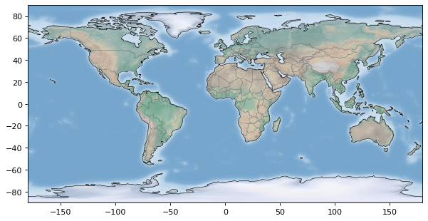
Draw a relief backdrop with coastlines and country borders on a global lon/lat (EPSG:4326) map:

import matplotlib
matplotlib.use("Agg")  # any backend; Agg shown for headless rendering
import matplotlib.pyplot as plt

from cleopatra.basemap.reference import add_relief, add_features

fig, ax = plt.subplots(figsize=(8, 4))
ax.set_xlim(-180, 180)
ax.set_ylim(-90, 90)
ax.set_aspect("equal")   # 1° lon == 1° lat, so the map is not stretched

add_relief(ax, resolution="low")                 # hypsometric backdrop
add_features(ax, "coastline", "110m", colors="black")
add_features(ax, "borders", "110m", colors="0.4")

fig.savefig("world.png", dpi=100)

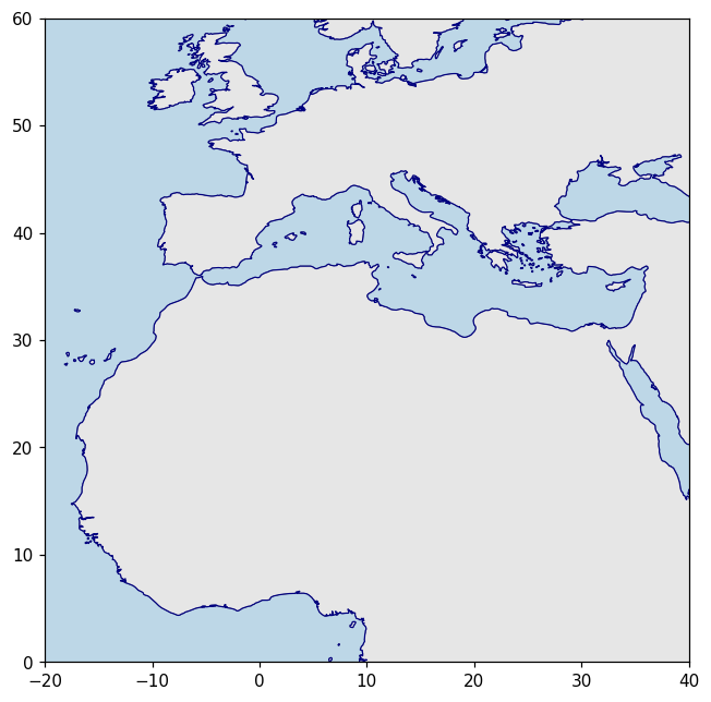
Relief backdrop with coastline and borders

A regional map with a filled land layer and higher-resolution coastline:

fig, ax = plt.subplots()
ax.set_xlim(-20, 40)   # Europe / N. Africa, in lon/lat
ax.set_ylim(0, 60)
ax.set_aspect("equal")

add_features(ax, "ocean", "50m", facecolors="#bdd7e7")
add_features(ax, "land", "50m", facecolors="0.9", edgecolors="0.5")
add_features(ax, "coastline", "50m", colors="navy", linewidths=0.8)

fig.savefig("europe.png")

Filled land and ocean over Europe and North Africa

If your data is in a projected CRS, pass crs= so the vectors are reprojected to match (requires pyproj):

add_features(ax, "coastline", "50m", crs=3857)   # Web Mercator axes

The raw data is also available without drawing:

from cleopatra.basemap.reference import natural_earth, natural_earth_polygons, relief

parts = natural_earth("coastline", "110m")   # list of (N, 2) lon/lat arrays
rgb = relief("low")                          # (H, W, 3) uint8 RGB array

natural_earth returns exterior rings only, which is right for line layers and polygon outlines. For a correct filled polygon on a non-matplotlib tier, use natural_earth_polygons(layer, resolution) on the polygon layers (land, ocean, lakes): it returns each polygon as [exterior_ring, *hole_rings], so ocean's continent-shaped holes and land's lake-shaped holes are preserved rather than filled over.

polys = natural_earth_polygons("ocean", "110m")   # list of [exterior, *holes]

To discover the valid arguments, call available_layers() and available_resolutions() for the vector layers, and available_relief_resolutions() for the relief products.

Note

add_features / add_relief read the axes' current xlim/ylim and preserve them, so plot your data first. Polygon layers (land/ocean/lakes) are drawn as a filled PathCollection with interior holes cut out (style with facecolors / edgecolors / linewidths); line layers (coastline/rivers/borders) as a LineCollection (style with colors / linewidths). Coordinates are EPSG:4326 unless you pass crs=. Set ax.set_aspect("equal") on lon/lat maps so degrees render at the same scale (matplotlib's default aspect="auto" otherwise stretches the map to fill the figure).

Caching

The first call downloads the asset from the cleopatra basemap-data-v1 release and caches it under ~/.cleopatra/naturalearth; subsequent calls work offline. Override the location with the CLEOPATRA_CACHE_DIR environment variable, or discover/resolve it programmatically with Config.get_cache_dir(). Downloads are restricted to http(s) URLs.

Migrating from `pyramids.basemap`#

This data used to live in pyramids.basemap (natural_earth / relief). It has moved to cleopatra.basemap.reference, which is the matplotlib map-decoration layer — the same boundary the web-tile basemaps already follow (pyramids.basemap forwarded to cleopatra.basemap.tiles). cleopatra hosts its own copy of the assets and has no dependency on pyramids.

Old (`pyramids.basemap`)	New (`cleopatra.basemap.reference`)	Notes
`natural_earth(layer, resolution)` → `FeatureCollection`	`natural_earth(layer, resolution)` → `list[np.ndarray]`	Now returns plain `(N, 2)` lon/lat arrays (exterior rings for polygons), not a GIS feature object.
`relief(resolution)` → GDAL `Dataset`	`relief(resolution)` → `(H, W, 3)` uint8 array	Now a NumPy RGB array; the asset is a PNG (no GeoTIFF / GDAL).
(draw it yourself)	`add_features(ax, layer, resolution)`	New axes helper — the `ax.coastlines()` analogue.
(draw it yourself)	`add_relief(ax, resolution)`	New axes helper — the `stock_img()` analogue.
`PYRAMIDS_CACHE_DIR`, `~/.pyramids/naturalearth`	`CLEOPATRA_CACHE_DIR`, `~/.cleopatra/naturalearth`	Cache env var and default directory renamed.

The pyramids.basemap.natural_earth / relief entry points are deprecated and emit a DeprecationWarning; update imports to cleopatra.basemap.reference. Resolutions are unchanged (110m / 50m / 10m for vectors; low / medium for relief), as are the six layer names.

Module Documentation #

`cleopatra.basemap.reference` #

Reference-basemap backdrops for matplotlib axes.

Two axes-level helpers that draw public cartographic reference data underneath your own plotted data -- the cartopy GeoAxes.stock_img() / ax.coastlines() niche, and the vector/raster sibling of cleopatra.basemap.tiles.add_tiles:

add_relief -- a global hypsometric relief image (the stock_img() analogue).
add_features -- a Natural Earth vector layer: coastline, borders, land, ocean, rivers, or lakes (the coastlines() analogue).

Both fetch a small, fixed public dataset that cleopatra re-hosts as a dependency-light artifact, cache it on disk, and render it with matplotlib. They acquire reference data only; they never read user files and never touch GDAL/geopandas:

Relief is re-hosted as a plain PNG, so decoding needs only Pillow (already part of the cleopatra[tiles] extra). Every relief product is a global EPSG:4326 raster, so its extent is hardcoded rather than read from a geotransform.
Natural Earth layers are pre-converted (offline, maintainer-side) to gzipped GeoJSON, so reading them needs only the standard library (json + gzip) plus numpy. Drawing in EPSG:4326 needs nothing beyond matplotlib; reprojecting to another CRS lazily uses pyproj (also in the [tiles] extra).

The cache directory defaults to ~/.cleopatra/naturalearth and can be overridden with the CLEOPATRA_CACHE_DIR environment variable; it is resolved by cleopatra.config.Config.get_cache_dir, where the setting is also discoverable. Downloads are restricted to http(s) URLs.

Examples:

Draw a relief backdrop and a coastline over data plotted in lon/lat (EPSG:4326):

>>> import matplotlib
>>> matplotlib.use("Agg")
>>> import matplotlib.pyplot as plt
>>> from cleopatra.basemap.reference import add_relief, add_features
>>> fig, ax = plt.subplots()
>>> ax.set_xlim(-20, 40); ax.set_ylim(0, 60)
>>> _ = add_relief(ax, resolution="low")
>>> _ = add_features(ax, "coastline", "50m")

`add_features(ax, layer='coastline', resolution='110m', *, crs=None, zorder=0, **style)` #

Draw a Natural Earth reference layer on an Axes.

The cartopy ax.coastlines() analogue. Polygon layers (land/ocean/lakes) are drawn hole-aware as a filled PathCollection (so ocean's continent cut-outs and islands-in-lakes render correctly); line layers (coastline/rivers/borders) as a LineCollection. The source data is EPSG:4326; pass crs to reproject the geometry into the axes' CRS (requires pyproj). The current axis limits are preserved.

Parameters:

Name	Type	Description	Default
`ax`	`Any`	A matplotlib `Axes` with data already plotted.	required
`layer`	`str`	One of `available_layers()`.	`'coastline'`
`resolution`	`str`	One of `available_resolutions()`.	`'110m'`
`crs`	`int \| str \| None`	CRS of the data on `ax`. `None` or `4326`/`"EPSG:4326"` draws the lon/lat coordinates directly; any other value reprojects from EPSG:4326 first.	`None`
`zorder`	`int`	Matplotlib draw order for the layer.	`0`
`**style`	`Any`	Overrides merged over the per-kind defaults and forwarded to the underlying collection. Use polygon keys for polygon layers (`facecolors`, `edgecolors`, `linewidths`) and line keys for line layers (`colors`, `linewidths`).	`{}`

Returns:

Type	Description
`Any`	matplotlib.axes.Axes: The same axes, for chaining.

Raises:

Type	Description
`TypeError`	If `ax` is not a matplotlib Axes.
`ValueError`	If `layer` or `resolution` is unknown, or `crs` is not a valid CRS.
`ImportError`	If `crs` requires reprojection but `pyproj` is not installed.
`ConnectionError`	If the asset must be downloaded and the fetch fails.

Examples:

Overlay a coastline and country borders on a lon/lat map (downloads each layer on first use, then caches it):

>>> import matplotlib
>>> matplotlib.use("Agg")
>>> import matplotlib.pyplot as plt
>>> from cleopatra.basemap.reference import add_features
>>> fig, ax = plt.subplots()
>>> ax.set_xlim(-20, 40); ax.set_ylim(0, 60)  # doctest: +SKIP
>>> ax = add_features(ax, "coastline", "50m", colors="navy")  # doctest: +SKIP
>>> ax = add_features(ax, "borders", "50m")  # doctest: +SKIP

Unknown layers are rejected before any download:

>>> import matplotlib
>>> matplotlib.use("Agg")
>>> import matplotlib.pyplot as plt
>>> from cleopatra.basemap.reference import add_features
>>> fig, ax = plt.subplots()
>>> add_features(ax, "countries")
Traceback (most recent call last):
    ...
ValueError: Unknown layer 'countries'. Choose from ['coastline', 'land', 'ocean', 'rivers', 'lakes', 'borders'].

Source code in src/cleopatra/basemap/reference.py

def add_features(
    ax: Any,
    layer: str = "coastline",
    resolution: str = "110m",
    *,
    crs: int | str | None = None,
    zorder: int = 0,
    **style: Any,
) -> Any:
    """Draw a Natural Earth reference layer on an Axes.

    The `cartopy` `ax.coastlines()` analogue. Polygon layers
    (`land`/`ocean`/`lakes`) are drawn hole-aware as a filled
    `PathCollection` (so `ocean`'s continent cut-outs and islands-in-lakes
    render correctly); line layers (`coastline`/`rivers`/`borders`) as a
    `LineCollection`. The source data is EPSG:4326; pass `crs` to reproject
    the geometry into the axes' CRS (requires `pyproj`). The current axis
    limits are preserved.

    Args:
        ax: A matplotlib `Axes` with data already plotted.
        layer: One of `available_layers()`.
        resolution: One of `available_resolutions()`.
        crs: CRS of the data on `ax`. `None` or `4326`/`"EPSG:4326"`
            draws the lon/lat coordinates directly; any other value
            reprojects from EPSG:4326 first.
        zorder: Matplotlib draw order for the layer.
        **style: Overrides merged over the per-kind defaults and
            forwarded to the underlying collection. Use polygon keys for
            polygon layers (`facecolors`, `edgecolors`, `linewidths`) and
            line keys for line layers (`colors`, `linewidths`).

    Returns:
        matplotlib.axes.Axes: The same axes, for chaining.

    Raises:
        TypeError: If `ax` is not a matplotlib Axes.
        ValueError: If `layer` or `resolution` is unknown, or `crs` is not
            a valid CRS.
        ImportError: If `crs` requires reprojection but `pyproj` is not
            installed.
        ConnectionError: If the asset must be downloaded and the fetch
            fails.

    Examples:
        - Overlay a coastline and country borders on a lon/lat map
            (downloads each layer on first use, then caches it):
            ```python
            >>> import matplotlib
            >>> matplotlib.use("Agg")
            >>> import matplotlib.pyplot as plt
            >>> from cleopatra.basemap.reference import add_features
            >>> fig, ax = plt.subplots()
            >>> ax.set_xlim(-20, 40); ax.set_ylim(0, 60)  # doctest: +SKIP
            >>> ax = add_features(ax, "coastline", "50m", colors="navy")  # doctest: +SKIP
            >>> ax = add_features(ax, "borders", "50m")  # doctest: +SKIP

            ```
        - Unknown layers are rejected before any download:
            ```python
            >>> import matplotlib
            >>> matplotlib.use("Agg")
            >>> import matplotlib.pyplot as plt
            >>> from cleopatra.basemap.reference import add_features
            >>> fig, ax = plt.subplots()
            >>> add_features(ax, "countries")
            Traceback (most recent call last):
                ...
            ValueError: Unknown layer 'countries'. Choose from ['coastline', 'land', 'ocean', 'rivers', 'lakes', 'borders'].

            ```
    """
    _validate_axes(ax)
    geoms = _load_features(layer, resolution)
    transformer = None if _is_4326(crs) else _make_transformer(crs)  # type: ignore[arg-type]

    kind = _LAYERS[layer][1]
    opts = {**_FEATURE_STYLE[kind], **style}

    xlim, ylim = ax.get_xlim(), ax.get_ylim()
    collection: Any
    if kind == "polygon":
        collection = PathCollection(
            _polygon_paths(geoms, transformer), zorder=zorder, **opts
        )
        collection.set_transform(ax.transData)
    else:
        collection = LineCollection(
            _line_segments(geoms, transformer), zorder=zorder, **opts
        )
    ax.add_collection(collection)
    ax.set_xlim(xlim)
    ax.set_ylim(ylim)
    return ax

`add_relief(ax, resolution='low', *, extent=None, alpha=1.0, zorder=-1, interpolation='bilinear', crs=None)` #

Draw a global hypsometric relief backdrop under existing data.

The cartopy GeoAxes.stock_img() analogue. Assumes the axes are in EPSG:4326 (lon/lat) unless crs says otherwise, in which case the relief is warped into that CRS. The current axis limits are preserved so adding the backdrop never changes the view.

Note

The relief image is equirectangular (EPSG:4326). On an EPSG:4326 axis (the default, crs=None) a lon/lat extent within the global bounds is cropped out of the global image and placed over that box, so a regional call shows that region's terrain rather than the whole world squashed into it (the recurring #177 footgun). The crop is placed at its snapped pixel edges so the terrain registers at true scale; the axis limits (preserved below) then clip to the requested view. extent=None places the whole globe. An extent OUTSIDE the global lon/lat bounds on a 4326 axis is instead stretched by imshow to fit -- visually acceptable for small extents but not a true reprojection.

For a non-EPSG:4326 crs the relief is warped into the axis CRS (per-pixel inverse reprojection via pyproj) so it lines up under data plotted in that CRS, exactly like add_features / add_tiles. The placement box defaults to the current axis view; parts of the box that fall outside the CRS's domain are left transparent. The box (and the axis view it defaults from) is assumed non-inverted -- west < east, south < north. This path needs pyproj (the [tiles] extra).

Parameters:

Name	Type	Description	Default
`ax`	`Any`	A matplotlib `Axes` with data already plotted (so its limits define the view).	required
`resolution`	`str`	`"low"` or `"medium"` (see `available_relief_resolutions`).	`'low'`
`extent`	`tuple[float, float, float, float] \| None`	`(west, south, east, north)` placement in axis units. On an EPSG:4326 axis, `None` (default) uses the whole global relief `(-180, -90, 180, 90)`, and a box within the global bounds is cropped out and placed at true scale (a regional view shows only that region); see `Note` for crop-vs-stretch. For a non-4326 `crs`, `None` fills the current axis view and any box is interpreted in the axis CRS's units.	`None`
`alpha`	`float`	Backdrop opacity in `[0, 1]`.	`1.0`
`zorder`	`int`	Matplotlib draw order (`-1` puts it behind all data).	`-1`
`interpolation`	`str`	Interpolation passed to `ax.imshow`.	`'bilinear'`
`crs`	`int \| str \| None`	CRS of the data on the axis. `None` or EPSG:4326 places the relief in lon/lat with no reprojection; any other CRS (int EPSG code or CRS string) warps the relief into it.	`None`

Returns:

Type	Description
`Any`	matplotlib.axes.Axes: The same axes, for chaining.

Raises:

Type	Description
`ImportError`	If Pillow (the `[tiles]` extra) is not installed, or if a non-EPSG:4326 `crs` is requested without pyproj (also `[tiles]`).
`TypeError`	If `ax` is not a matplotlib Axes.
`ValueError`	If `resolution` or `crs` is unknown.
`ConnectionError`	If the asset must be downloaded and the fetch fails.

Examples:

Draw a relief backdrop under data already plotted in lon/lat (downloads the asset on first use, then caches it):

>>> import matplotlib
>>> matplotlib.use("Agg")
>>> import matplotlib.pyplot as plt
>>> from cleopatra.basemap.reference import add_relief
>>> fig, ax = plt.subplots()
>>> ax.set_xlim(-180, 180); ax.set_ylim(-90, 90)  # doctest: +SKIP
>>> ax = add_relief(ax, "low")  # doctest: +SKIP
>>> len(ax.images)  # doctest: +SKIP
1

Unknown resolutions are rejected before any download:

>>> import matplotlib
>>> matplotlib.use("Agg")
>>> import matplotlib.pyplot as plt
>>> from cleopatra.basemap.reference import add_relief
>>> fig, ax = plt.subplots()
>>> add_relief(ax, "high")
Traceback (most recent call last):
    ...
ValueError: Unknown relief resolution 'high'. Choose from ['low', 'medium'].

Source code in src/cleopatra/basemap/reference.py

def add_relief(
    ax: Any,
    resolution: str = "low",
    *,
    extent: tuple[float, float, float, float] | None = None,
    alpha: float = 1.0,
    zorder: int = -1,
    interpolation: str = "bilinear",
    crs: int | str | None = None,
) -> Any:
    """Draw a global hypsometric relief backdrop under existing data.

    The `cartopy` `GeoAxes.stock_img()` analogue. Assumes the axes are in
    EPSG:4326 (lon/lat) unless `crs` says otherwise, in which case the relief
    is warped into that CRS. The current axis limits are preserved so adding
    the backdrop never changes the view.

    Note:
        The relief image is equirectangular (EPSG:4326). On an EPSG:4326 axis
        (the default, `crs=None`) a lon/lat `extent` within the global bounds
        is **cropped** out of the global image and placed over that box, so a
        regional call shows that region's terrain rather than the whole world
        squashed into it (the recurring #177 footgun). The crop is placed at
        its **snapped pixel edges** so the terrain registers at true scale; the
        axis limits (preserved below) then clip to the requested view.
        `extent=None` places the whole globe. An `extent` OUTSIDE the global
        lon/lat bounds on a 4326 axis is instead stretched by `imshow` to fit
        -- visually acceptable for small extents but not a true reprojection.

        For a **non-EPSG:4326 `crs`** the relief is **warped** into the axis
        CRS (per-pixel inverse reprojection via pyproj) so it lines up under
        data plotted in that CRS, exactly like `add_features` / `add_tiles`.
        The placement box defaults to the current axis view; parts of the box
        that fall outside the CRS's domain are left transparent. The box (and
        the axis view it defaults from) is assumed non-inverted -- `west <
        east`, `south < north`. This path needs pyproj (the `[tiles]` extra).

    Args:
        ax: A matplotlib `Axes` with data already plotted (so its limits
            define the view).
        resolution: `"low"` or `"medium"` (see
            `available_relief_resolutions`).
        extent: `(west, south, east, north)` placement in axis units. On an
            EPSG:4326 axis, `None` (default) uses the whole global relief
            `(-180, -90, 180, 90)`, and a box within the global bounds is
            cropped out and placed at true scale (a regional view shows only
            that region); see `Note` for crop-vs-stretch. For a non-4326 `crs`,
            `None` fills the current axis view and any box is interpreted in the
            axis CRS's units.
        alpha: Backdrop opacity in `[0, 1]`.
        zorder: Matplotlib draw order (`-1` puts it behind all data).
        interpolation: Interpolation passed to `ax.imshow`.
        crs: CRS of the data on the axis. `None` or EPSG:4326 places the
            relief in lon/lat with no reprojection; any other CRS (int EPSG
            code or CRS string) warps the relief into it.

    Returns:
        matplotlib.axes.Axes: The same axes, for chaining.

    Raises:
        ImportError: If Pillow (the `[tiles]` extra) is not installed, or if
            a non-EPSG:4326 `crs` is requested without pyproj (also `[tiles]`).
        TypeError: If `ax` is not a matplotlib Axes.
        ValueError: If `resolution` or `crs` is unknown.
        ConnectionError: If the asset must be downloaded and the fetch
            fails.

    Examples:
        - Draw a relief backdrop under data already plotted in lon/lat
            (downloads the asset on first use, then caches it):
            ```python
            >>> import matplotlib
            >>> matplotlib.use("Agg")
            >>> import matplotlib.pyplot as plt
            >>> from cleopatra.basemap.reference import add_relief
            >>> fig, ax = plt.subplots()
            >>> ax.set_xlim(-180, 180); ax.set_ylim(-90, 90)  # doctest: +SKIP
            >>> ax = add_relief(ax, "low")  # doctest: +SKIP
            >>> len(ax.images)  # doctest: +SKIP
            1

            ```
        - Unknown resolutions are rejected before any download:
            ```python
            >>> import matplotlib
            >>> matplotlib.use("Agg")
            >>> import matplotlib.pyplot as plt
            >>> from cleopatra.basemap.reference import add_relief
            >>> fig, ax = plt.subplots()
            >>> add_relief(ax, "high")
            Traceback (most recent call last):
                ...
            ValueError: Unknown relief resolution 'high'. Choose from ['low', 'medium'].

            ```
    """
    _validate_axes(ax)
    rgb = relief(resolution)
    xlim, ylim = ax.get_xlim(), ax.get_ylim()
    if _is_4326(crs):
        if extent is None:
            west, south, east, north = _RELIEF_EXTENT_4326
        else:
            west, south, east, north = extent
            gw, gs, ge, gn = _RELIEF_EXTENT_4326
            if gw <= west < east <= ge and gs <= south < north <= gn:
                rows, cols = rgb.shape[:2]
                c0 = max(0, int(np.floor((west - gw) / (ge - gw) * cols)))
                c1 = min(
                    cols, max(c0 + 1, int(np.ceil((east - gw) / (ge - gw) * cols)))
                )
                r0 = max(0, int(np.floor((gn - north) / (gn - gs) * rows)))
                r1 = min(
                    rows, max(r0 + 1, int(np.ceil((gn - south) / (gn - gs) * rows)))
                )
                rgb = rgb[r0:r1, c0:c1]
                west = gw + c0 / cols * (ge - gw)
                east = gw + c1 / cols * (ge - gw)
                north = gn - r0 / rows * (gn - gs)
                south = gn - r1 / rows * (gn - gs)
        ax.imshow(
            rgb,
            extent=[west, east, south, north],
            origin="upper",
            alpha=alpha,
            zorder=zorder,
            interpolation=interpolation,
            aspect=ax.get_aspect(),
        )
    else:
        if extent is None:
            west, east = xlim
            south, north = ylim
        else:
            west, south, east, north = extent
        warped = _warp_relief(rgb, (west, south, east, north), crs, alpha)  # type: ignore[arg-type]
        ax.imshow(
            warped,
            extent=[west, east, south, north],
            origin="upper",
            zorder=zorder,
            interpolation=interpolation,
            aspect=ax.get_aspect(),
        )
    ax.set_xlim(xlim)
    ax.set_ylim(ylim)
    return ax

`available_layers()` #

Return the Natural Earth layers that can be requested.

Returns:

Type	Description
`list[str]`	list[str]: Valid `layer` names for `natural_earth` / `add_features`.

Examples:

>>> from cleopatra.basemap.reference import available_layers
>>> available_layers()
['coastline', 'land', 'ocean', 'rivers', 'lakes', 'borders']

Source code in src/cleopatra/basemap/reference.py

def available_layers() -> list[str]:
    """Return the Natural Earth layers that can be requested.

    Returns:
        list[str]: Valid `layer` names for `natural_earth` /
            `add_features`.

    Examples:
        ```python
        >>> from cleopatra.basemap.reference import available_layers
        >>> available_layers()
        ['coastline', 'land', 'ocean', 'rivers', 'lakes', 'borders']

        ```
    """
    return list(_LAYERS)

`available_relief_resolutions()` #

Return the relief resolutions that can be requested.

Returns:

Type	Description
`list[str]`	list[str]: The valid `resolution` values for `relief` / `add_relief` (`"low"`, `"medium"`).

Examples:

>>> from cleopatra.basemap.reference import available_relief_resolutions
>>> available_relief_resolutions()
['low', 'medium']

Source code in src/cleopatra/basemap/reference.py

def available_relief_resolutions() -> list[str]:
    """Return the relief resolutions that can be requested.

    Returns:
        list[str]: The valid `resolution` values for `relief` /
            `add_relief` (`"low"`, `"medium"`).

    Examples:
        ```python
        >>> from cleopatra.basemap.reference import available_relief_resolutions
        >>> available_relief_resolutions()
        ['low', 'medium']

        ```
    """
    return list(_RELIEF_PRODUCTS)

`available_resolutions()` #

Return the supported Natural Earth resolutions.

Returns:

Type	Description
`list[str]`	list[str]: `["110m", "50m", "10m"]`.

Examples:

>>> from cleopatra.basemap.reference import available_resolutions
>>> available_resolutions()
['110m', '50m', '10m']

Source code in src/cleopatra/basemap/reference.py

def available_resolutions() -> list[str]:
    """Return the supported Natural Earth resolutions.

    Returns:
        list[str]: `["110m", "50m", "10m"]`.

    Examples:
        ```python
        >>> from cleopatra.basemap.reference import available_resolutions
        >>> available_resolutions()
        ['110m', '50m', '10m']

        ```
    """
    return list(_RESOLUTIONS)

`natural_earth(layer='coastline', resolution='110m')` #

Fetch (and cache) a Natural Earth layer as coordinate arrays.

The layer is downloaded as preprocessed gzipped GeoJSON and parsed with the standard library only -- no GDAL/geopandas. Coordinates are EPSG:4326 lon/lat. Polygon layers return exterior rings only; use natural_earth_polygons for hole-aware coordinate data, or add_features for hole-aware filled rendering.

Parameters:

Name	Type	Description	Default
`layer`	`str`	One of `available_layers()`.	`'coastline'`
`resolution`	`str`	One of `available_resolutions()` (`"110m"`/`"50m"`/`"10m"`).	`'110m'`

Returns:

Type	Description
`list[ndarray]`	list[numpy.ndarray]: One `(N, 2)` lon/lat array per geometry part (exterior rings for polygon layers).

Raises:

Type	Description
`ValueError`	If `layer` or `resolution` is unknown.
`ConnectionError`	If the asset must be downloaded and the fetch fails.

Examples:

Fetch coastlines and inspect the parts (downloads on first use, then reads from the cache):

>>> from cleopatra.basemap.reference import natural_earth
>>> parts = natural_earth("coastline", "110m")  # doctest: +SKIP
>>> parts[0].shape[1]  # each part is an (N, 2) lon/lat array  # doctest: +SKIP
2

Unknown layers are rejected before any download:

>>> from cleopatra.basemap.reference import natural_earth
>>> natural_earth("countries")
Traceback (most recent call last):
    ...
ValueError: Unknown layer 'countries'. Choose from ['coastline', 'land', 'ocean', 'rivers', 'lakes', 'borders'].

Source code in src/cleopatra/basemap/reference.py

def natural_earth(
    layer: str = "coastline", resolution: str = "110m"
) -> list[np.ndarray]:
    """Fetch (and cache) a Natural Earth layer as coordinate arrays.

    The layer is downloaded as preprocessed gzipped GeoJSON and parsed
    with the standard library only -- no GDAL/geopandas. Coordinates are
    EPSG:4326 lon/lat. Polygon layers return exterior rings only; use
    `natural_earth_polygons` for hole-aware coordinate data, or `add_features`
    for hole-aware filled rendering.

    Args:
        layer: One of `available_layers()`.
        resolution: One of `available_resolutions()`
            (`"110m"`/`"50m"`/`"10m"`).

    Returns:
        list[numpy.ndarray]: One `(N, 2)` lon/lat array per geometry part
            (exterior rings for polygon layers).

    Raises:
        ValueError: If `layer` or `resolution` is unknown.
        ConnectionError: If the asset must be downloaded and the fetch
            fails.

    Examples:
        - Fetch coastlines and inspect the parts (downloads on first use,
            then reads from the cache):
            ```python
            >>> from cleopatra.basemap.reference import natural_earth
            >>> parts = natural_earth("coastline", "110m")  # doctest: +SKIP
            >>> parts[0].shape[1]  # each part is an (N, 2) lon/lat array  # doctest: +SKIP
            2

            ```
        - Unknown layers are rejected before any download:
            ```python
            >>> from cleopatra.basemap.reference import natural_earth
            >>> natural_earth("countries")
            Traceback (most recent call last):
                ...
            ValueError: Unknown layer 'countries'. Choose from ['coastline', 'land', 'ocean', 'rivers', 'lakes', 'borders'].

            ```
    """
    parts: list[np.ndarray] = []
    for geometry in _load_features(layer, resolution):
        parts.extend(_paths(geometry))
    return parts

`natural_earth_polygons(layer, resolution='110m')` #

Fetch (and cache) a Natural Earth polygon layer as hole-aware rings.

The engine-neutral data analogue of add_features: where natural_earth returns one flat (N, 2) array per part and keeps exterior rings only, this returns each polygon as [exterior_ring, *hole_rings], so a consumer that is not matplotlib (a web/MapLibre tier, a 3-D tier, a GeoJSON builder) can draw a correct filled polygon. The holes matter: ocean polygons carry continent-shaped holes and land polygons carry lake-shaped holes, so a fill built from exterior rings alone paints over them.

Only the polygon layers (land, ocean, lakes) are accepted; the line layers (coastline, rivers, borders) have no fillable interior, so use natural_earth for those. Coordinates are EPSG:4326 lon/lat and the ring winding is the source GeoJSON's (not normalised); a renderer that needs a specific winding should orient the rings itself, as add_features does.

Parameters:

Name	Type	Description	Default
`layer`	`str`	One of the polygon layers in `available_layers()` -- `"land"`, `"ocean"`, or `"lakes"`.	required
`resolution`	`str`	One of `available_resolutions()` (`"110m"`/`"50m"`/`"10m"`).	`'110m'`

Returns:

Type	Description
`list[list[ndarray]]`	list[list[numpy.ndarray]]: One entry per polygon part; each entry is `[exterior_ring, *hole_rings]` of `(N, 2)` lon/lat arrays. A polygon with no holes is a single-element list `[exterior_ring]`.

Raises:

Type	Description
`ValueError`	If `layer` is unknown, or is a line layer rather than a polygon layer; or if `resolution` is unknown.
`ConnectionError`	If the asset must be downloaded and the fetch fails.

Examples:

Fetch ocean polygons hole-aware (downloads on first use, then reads from the cache); the 110m ocean comes back as two parts -- a small hole-free polygon and the main ocean, which carries one exterior ring plus a hole per landmass:

>>> from cleopatra.basemap.reference import natural_earth_polygons
>>> polys = natural_earth_polygons("ocean", "110m")  # doctest: +SKIP
>>> [len(rings) for rings in polys]  # [exterior, *holes] per part  # doctest: +SKIP
[1, 121]

Line layers have no fillable interior and are rejected before any download:

>>> from cleopatra.basemap.reference import natural_earth_polygons
>>> natural_earth_polygons("coastline")
Traceback (most recent call last):
    ...
ValueError: Layer 'coastline' is a line layer, not a polygon layer; use natural_earth for it. Polygon layers: ['land', 'ocean', 'lakes'].

Source code in src/cleopatra/basemap/reference.py

def natural_earth_polygons(
    layer: str, resolution: str = "110m"
) -> list[list[np.ndarray]]:
    """Fetch (and cache) a Natural Earth polygon layer as hole-aware rings.

    The engine-neutral data analogue of `add_features`: where `natural_earth`
    returns one flat `(N, 2)` array per part and keeps exterior rings only, this
    returns each polygon as `[exterior_ring, *hole_rings]`, so a consumer that is
    not matplotlib (a web/MapLibre tier, a 3-D tier, a GeoJSON builder) can draw
    a correct filled polygon. The holes matter: ocean polygons carry
    continent-shaped holes and land polygons carry lake-shaped holes, so a fill
    built from exterior rings alone paints over them.

    Only the polygon layers (`land`, `ocean`, `lakes`) are accepted; the line
    layers (`coastline`, `rivers`, `borders`) have no fillable interior, so use
    `natural_earth` for those. Coordinates are EPSG:4326 lon/lat and the ring
    winding is the source GeoJSON's (not normalised); a renderer that needs a
    specific winding should orient the rings itself, as `add_features` does.

    Args:
        layer: One of the polygon layers in `available_layers()` -- `"land"`,
            `"ocean"`, or `"lakes"`.
        resolution: One of `available_resolutions()`
            (`"110m"`/`"50m"`/`"10m"`).

    Returns:
        list[list[numpy.ndarray]]: One entry per polygon part; each entry is
            `[exterior_ring, *hole_rings]` of `(N, 2)` lon/lat arrays. A
            polygon with no holes is a single-element list `[exterior_ring]`.

    Raises:
        ValueError: If `layer` is unknown, or is a line layer rather than a
            polygon layer; or if `resolution` is unknown.
        ConnectionError: If the asset must be downloaded and the fetch fails.

    Examples:
        - Fetch ocean polygons hole-aware (downloads on first use, then reads
            from the cache); the 110m ocean comes back as two parts -- a small
            hole-free polygon and the main ocean, which carries one exterior
            ring plus a hole per landmass:
            ```python
            >>> from cleopatra.basemap.reference import natural_earth_polygons
            >>> polys = natural_earth_polygons("ocean", "110m")  # doctest: +SKIP
            >>> [len(rings) for rings in polys]  # [exterior, *holes] per part  # doctest: +SKIP
            [1, 121]

            ```
        - Line layers have no fillable interior and are rejected before any
            download:
            ```python
            >>> from cleopatra.basemap.reference import natural_earth_polygons
            >>> natural_earth_polygons("coastline")
            Traceback (most recent call last):
                ...
            ValueError: Layer 'coastline' is a line layer, not a polygon layer; use natural_earth for it. Polygon layers: ['land', 'ocean', 'lakes'].

            ```
    """
    kind = _LAYERS.get(layer, (None, None))[1]
    if kind is not None and kind != "polygon":
        polygon_layers = [name for name, (_, k) in _LAYERS.items() if k == "polygon"]
        raise ValueError(
            f"Layer {layer!r} is a {kind} layer, not a polygon layer; use "
            f"natural_earth for it. Polygon layers: {polygon_layers}."
        )
    polygons: list[list[np.ndarray]] = []
    for geometry in _load_features(layer, resolution):
        polygons.extend(_polygons(geometry))
    return polygons

`relief(resolution='low')` #

Fetch (and cache) a hypsometric relief product as an RGB array.

Parameters:

Name	Type	Description	Default
`resolution`	`str`	`"low"` (720x360) or `"medium"` (1440x720).	`'low'`

Returns:

Type	Description
`ndarray`	numpy.ndarray: An `(H, W, 3)` uint8 RGB array in EPSG:4326, north-up (row 0 is the northern edge).

Raises:

Type	Description
`ImportError`	If Pillow (the `[tiles]` extra) is not installed.
`ValueError`	If `resolution` is not a known product.
`ConnectionError`	If the asset must be downloaded and the fetch fails.
`OSError`	If the cached file cannot be decoded as an image (the poisoned file is removed first so a retry re-downloads).

Examples:

Unknown resolutions raise ValueError before any download:

>>> from cleopatra.basemap.reference import relief
>>> relief("ultra")
Traceback (most recent call last):
    ...
ValueError: Unknown relief resolution 'ultra'. Choose from ['low', 'medium'].

Source code in src/cleopatra/basemap/reference.py

def relief(resolution: str = "low") -> np.ndarray:
    """Fetch (and cache) a hypsometric relief product as an RGB array.

    Args:
        resolution: `"low"` (720x360) or `"medium"` (1440x720).

    Returns:
        numpy.ndarray: An `(H, W, 3)` uint8 RGB array in EPSG:4326,
            north-up (row 0 is the northern edge).

    Raises:
        ImportError: If Pillow (the `[tiles]` extra) is not installed.
        ValueError: If `resolution` is not a known product.
        ConnectionError: If the asset must be downloaded and the fetch
            fails.
        OSError: If the cached file cannot be decoded as an image (the
            poisoned file is removed first so a retry re-downloads).

    Examples:
        - Unknown resolutions raise `ValueError` before any download:
            ```python
            >>> from cleopatra.basemap.reference import relief
            >>> relief("ultra")
            Traceback (most recent call last):
                ...
            ValueError: Unknown relief resolution 'ultra'. Choose from ['low', 'medium'].

            ```
    """
    if resolution not in _RELIEF_PRODUCTS:
        raise ValueError(
            f"Unknown relief resolution {resolution!r}. "
            f"Choose from {available_relief_resolutions()}."
        )
    if not _PILLOW_AVAILABLE:
        raise ImportError(_PILLOW_HINT)
    from PIL import Image, UnidentifiedImageError

    name = _RELIEF_PRODUCTS[resolution]
    path = _download(_RELIEF_BASE_URL + name, _cache_dir() / name)
    try:
        with Image.open(path) as img:
            return np.asarray(img.convert("RGB"))
    except (UnidentifiedImageError, OSError, ValueError) as e:
        path.unlink(missing_ok=True)
        raise OSError(
            f"Cached relief asset {path} could not be decoded ({e}); removed "
            "it -- retry to re-download."
        ) from e